Coverage probability

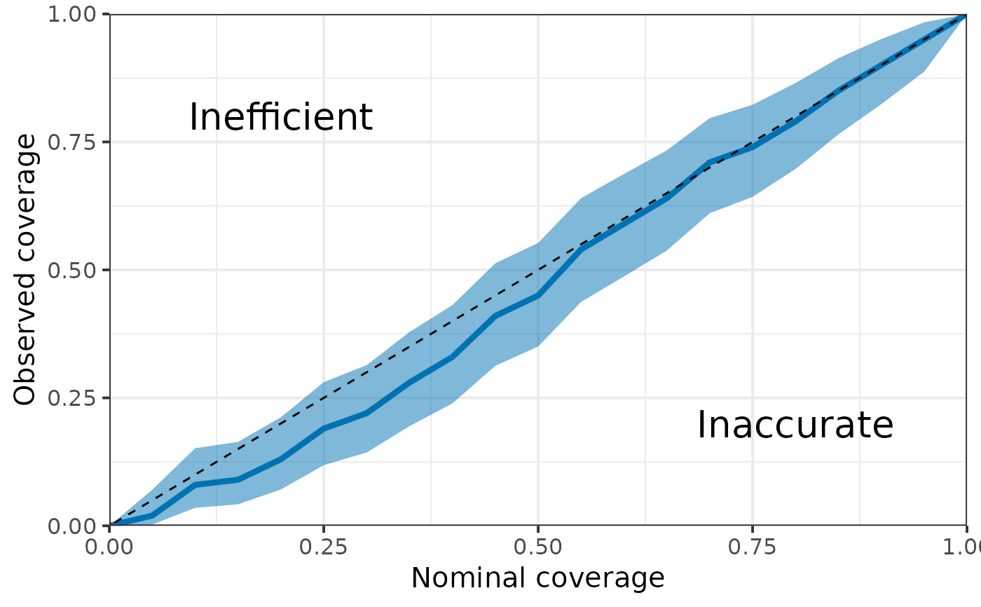
Compute and plot coverage of CI for different confidence level. Useful for fake data check.

Usage

compute_coverage(
  post_samples,
  truth,
  CI = seq(0, 1, 0.05),
  type = c("eti", "hdi")
)

plot_coverage(
  post_samples,
  truth,
  CI = seq(0, 1, 0.05),
  type = c("eti", "hdi")
)

Arguments

post_samples

Matrix of posterior samples. Rows represent a sample and columns represent variables.

truth

Vector of true parameter values (should be the same length as the number of columns in post_samples).

CI

Vector of confidence levels.

type

Type of confidence intervals: either "eti" (equal-tailed intervals) or "hdi" (highest density intervals).

Value

compute_coverage returns a Dataframe containing coverage (and 95% uncertainty interval for the coverage) for different confidence level (nominal coverage). plot_coverage returns a ggplot of the coverage as the function of the nominal coverage with 95% uncertainty interval.

Examples

N <- 100
N_post <- 1e3
truth <- rep(0, N)
post_samples <- sapply(rnorm(N, 0, 1), function(x) {
  rnorm(N_post, x, 1)
})

compute_coverage(post_samples, truth)
#> # A tibble: 21 × 4
#>    Nominal Coverage  Lower  Upper
#>      <dbl>    <dbl>  <dbl>  <dbl>
#>  1    0        0    0      0     
#>  2    0.05     0.04 0.0110 0.0993
#>  3    0.1      0.09 0.0420 0.164 
#>  4    0.15     0.17 0.102  0.258 
#>  5    0.2      0.22 0.143  0.314 
#>  6    0.25     0.3  0.212  0.400 
#>  7    0.3      0.32 0.230  0.421 
#>  8    0.35     0.38 0.285  0.483 
#>  9    0.4      0.42 0.322  0.523 
#> 10    0.45     0.49 0.389  0.592 
#> # ℹ 11 more rows
plot_coverage(post_samples, truth)