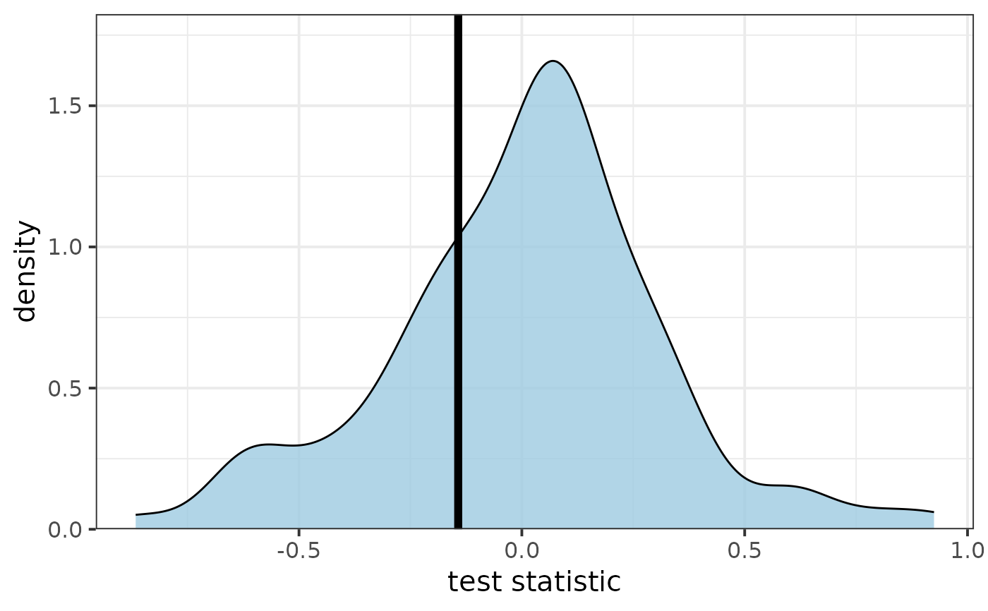
Posterior Predictive p-value — post_pred

Compute and plot posterior predictive p-value (Bayesian p-value) from samples of a distribution. The simulations and observations are first summarised into a test statistics, then the test statistic of the observations is compared to the test statistic of the empirical distribution.

post_pred_pval(
  yrep,
  y,
  test_statistic = mean,
  alternative = c("two.sided", "less", "greater"),
  plot = FALSE
)

Arguments

yrep: Matrix of posterior replications with rows corresponding to samples and columns to simulated observations.
y: Vector of observations.
test_statistic: Function of the test statistic to compute the p-value for.
alternative: Indicates the alternative hypothesis: must be one of "two.sided", "greater" or "less".
plot: Whether to output a plot visualising the distribution of the test statistic.

Value

List containing the p-value and (optionally) a ggplot.

Examples

post_pred_pval(matrix(rnorm(1e3), ncol = 10), rnorm(10), plot = TRUE)
#> $pval
#> [1] 0.5742574
#> 
#> $plot

#>